Investing in an emerging supplier to encourage product innovation under market competition and R&D uncertainty

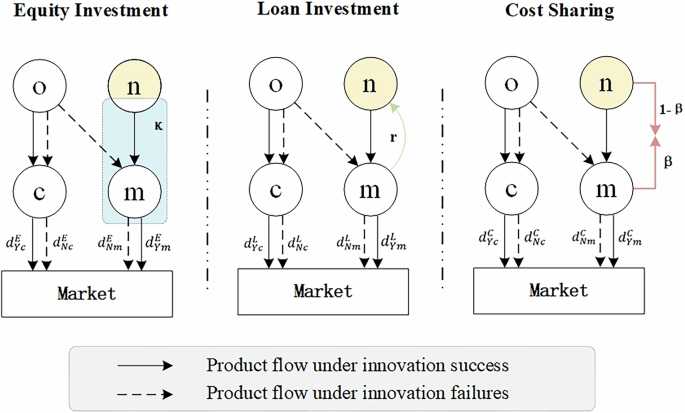
In this section, we first introduce the equilibrium results under different strategies. Then, we explore the conditions under which it is profitable for the manufacturer to invest in the emerging supplier. Based on this, we provide a sensitivity analysis and comparison of relevant parameters under different investment strategies when the manufacturer invests in the emerging supplier. Next, we discuss the strategy preferences of supply chain members under different investment strategies. Finally, we compare consumer surplus and social welfare under different investment strategies.

Equilibrium results

First, we consider the decision-making process of the manufacturer when choosing to invest in the emerging supplier. In Strategy Z, the emerging supplier first decides the extent of product improvement through R&D. At this point, the optimization problem under different investment strategies is:

Among them, \({E[\pi }_{n}^{Z}]\) represents the expected profit of the emerging supplier when the manufacturer chooses the Z strategy, while the first term on the right side of the equation represents the expected profit when the emerging supplier’s product development is successful, and the second term represents the product development expenditure of the emerging supplier.

Then, the emerging supplier and the established supplier simultaneously decide the wholesale prices for the given downstream manufacturers. At this point, the optimization problem under different investment strategies is:

Among them, \({E[\pi }_{o}^{Z}]\) represents the expected profit of the established supplier when the manufacturer chooses the Z strategy, while the first term on the right side of the equation represents the expected profit of the established supplier when the emerging supplier’s product development is successful, and the second term represents the expected profit of the established supplier when the emerging supplier’s product development fails.

Finally, the manufacturer and its competitors simultaneously decide the retail price of the product. At this point, the optimization problem under different investment strategies is:

Among them, \({E[\pi }_{m}^{Z}]\) and \({E[\pi }_{c}^{Z}]\) represent the expected profits of the manufacturer and its competitor, respectively. The first term on the right side of the equation represents the expected profit for the manufacturers when the emerging supplier’s product development is successful, the second term represents the expected profit for the manufacturers when the emerging supplier’s product development fails, and the third term represents the gains or expenditures when the manufacturer chooses different investment strategies.

When the manufacturer chooses not to invest in the emerging supplier, that is, in strategy N, the established supplier first decides the wholesale prices for downstream enterprises, and then the manufacturer and their competitor respectively decide the retail prices for the products. Since the profit function expressions for the game participants are relatively simple and can be given by the above equations, they will not be repeated.

Based on the above analysis, the equilibrium results and expected profits of upstream and downstream enterprises in the supply chain can be obtained through backward induction. The specific calculation process is detailed in the appendix, and the detailed expressions of each equilibrium result are shown in Table A1. To ensure the non-negativity of the research results and to avoid other trivial situations, we need \(0 \,<\, b\, <\, \bar{b}\). Furthermore, before discussing the different investment strategies of the manufacturer, we first need to clarify the conditions under which it is profitable for the manufacturer to invest in the emerging supplier, thereby ensuring that all subsequent analyses are feasible. This leads to Proposition 1.

Proposition 1. There exists a threshold \({\underline{b}}\, > \,0\) such that the manufacturer m chooses to invest in the emerging supplier n if and only if \(b\le {\underline{b}}\), as shown in Fig. 3.

Conditions for the manufacturer to invest profitably in the emerging supplier.

Proposition 1 indicates that when \(b\) exceeds a certain threshold, the manufacturer has no incentive to invest in the emerging supplier, but instead chooses to share an established supplier with a competitor. This is because, in highly competitive markets, the manufacturer prefers to maintain the stability of their existing supply chains, avoiding the uncertainties brought by investing in the emerging supplier, as shown in the white area of Fig. 3. When \(b\) is below a certain threshold, the manufacturer will choose to invest in the emerging supplier, as shown in the red area of Fig. 3.The reason lies in the fact that under lower competitive pressure, the manufacturer has more room to pursue higher profits and product innovation (de Bettignies et al. 2023). Investing in the emerging supplier can help the manufacturer gain unique technological advantages and more flexible supply chains, thereby achieving differentiated competitiveness in the market. Moreover, lower \(b\) also means that the market’s sensitivity to price may be lower, allowing the manufacturer to achieve higher profits through innovative products rather than merely relying on price competition. In such a market environment, the manufacturer tends to adopt more aggressive investment strategies, aiming to develop more innovative products in collaboration with the emerging supplier, thereby increasing market share and brand value. Therefore, we focus on the case when \(b\le {\underline{b}}\) in the following analysis.

Note: the following parameter values are used: \(\kappa =0.49,\beta =0.05\)

Price and product improvement analysis

Lemma 1. The impact of \(b\) and \(\theta\) on prices.

Lemma 1 (a) indicates that both wholesale and retail prices of products decrease with the increase in market competition intensity. This is also consistent with the traditional view that fierce market competition often forces enterprises to attract and retain consumers through price adjustment, thus forming an overall trend of price decline (He et al. 2019). Like the intensity of market competition, the probability of R&D success also hurts the price, as shown in Lemma 1(b). As the probability of R&D success increases, the wholesale price of both suppliers will decrease. This is because the increase in the probability of R&D success not only intensifies the competition among suppliers but also enhances the bargaining power of manufacturers, thus adjusting market expectations. Under the combined action of these factors, the established supplier and the emerging supplier must reduce wholesale prices to provide more favorable purchasing conditions to expand their market share. For manufacturers, the increased probability of R&D success will also intensify competition, and the reduction of wholesale prices means that manufacturers have more profit margins, so they have enough incentive to reduce retail prices (Zhang et al. 2024). For example, in the home appliance industry, as the maturity of OLED technology enables TV manufacturers to produce thinner and more colorful screens, while increasing the yield of production, the competition between brands such as Samsung, LG, SONY, etc., has become increasingly fierce, resulting in the wholesale and retail prices of TV sets are falling (PConline 2015).

Lemma 2. The effect of \(b\) and \(\theta\) on the degree of product innovation.

Lemma 2(a) indicates that the degree of product improvement by the emerging supplier will increase with the intensity of market competition, but this effect will vary depending on the investment model. Specifically, under LI, the emerging supplier needs to bear higher financial risks and the pressure of repaying loans on their own. To avoid potential financial difficulties, the emerging supplier often tends to choose low-risk R&D projects, thereby suppressing the potential for product improvement. Under EI and CS, the manufacturer can share some of the R&D risks with the emerging supplier, motivating them to pursue product innovation (Zhang and Lee 2022). At the same time, while a high probability of successful R&D can facilitate the launch of new products, it may lead enterprises to adopt more conservative R&D strategies, thereby reducing the extent of improvements. This phenomenon seems counterintuitive, but it can be understood in this way: although a high success rate in R&D is beneficial for the launch of new products, it does not necessarily indicate a significant improvement in product quality. On one hand, a high probability of R&D success often means that the company has adopted a relatively conservative strategy during the R&D process, which may sacrifice a certain degree of innovation and breakthroughs (Lévesque 2000). Additionally, a high probability of success may also trigger incentive compatibility issues. In situations where the likelihood of success is high, the supplier might reduce their extra efforts because they believe that even without significant improvements, successful R&D is still possible. This behavior further diminishes the extent of product improvement. Therefore, to address the challenges, enterprises need to balance market competition and R&D risks through appropriate investment models and incentive mechanisms. Manufacturers, should choose suitable investment models based on the intensity of market competition and incentivize suppliers to innovate through risk-sharing mechanisms; meanwhile, suppliers need to find a balance between innovation and stability to achieve optimal R&D investment strategies. At the same time, enterprises in R&D management should avoid excessively pursuing R&D success rates and can encourage moderate high-risk R&D activities to drive more significant product improvements.

Lemma 3. The impact of other key parameters on wholesale prices, product prices, and product innovation, as shown in Table 3.

Lemma 3 shows that the shareholding under EI and the share ratio under CS have the same influence on the product price and the product innovation degree. With the increase in shareholding (share) ratio, the wholesale price of the emerging supplier, the retail price of the competitor, and the innovation degree of products will increase, the wholesale price of the established supplier will decrease, and the change of the manufacturer’s retail price will be affected by the success rate of R&D. The reason for this is that a higher shareholding (share) ratio means a closer cooperative relationship between the manufacturer and the emerging supplier, which increases the incentive for both parties to jointly invest in product innovation (Guo et al. 2024). In addition, as the degree of cooperation deepens, the emerging supplier may have access to more resources and technical support, which also helps them raise the price of their products. However, this strategy may also lead the established supplier to lower the wholesale prices of their products to remain competitive in the market, as they may face greater competitive pressure from the emerging supplier. The manufacturer, will adjust retail prices according to the success rate of R&D. If a higher R&D success rate indicates that product innovation from the emerging supplier is more likely to be successful, the manufacturer will raise retail prices to reflect the improvements and added value. Conversely, if R&D success rates are low, the manufacturer will lower retail prices to attract consumers and maintain market share.

Different from the above two strategies, with the increase of loan interest rate, the wholesale price of the emerging supplier, the retail price of the competitor, and the innovation degree of products will decrease, while the wholesale price of the established supplier will increase, and the change of the manufacturer’s retail price is still related to the success rate of R&D. This is because the loan investment increases the financial pressure on the emerging supplier, placing them solely responsible for the repayment of loans and the risk of R&D failure, so they invest less in product innovation. This financial pressure is further exacerbated by higher lending rates, which lead to lower wholesale prices and product innovation for the emerging supplier. At this time, since the products of the emerging supplier are not very competitive, the established supplier may take advantage of this to raise their wholesale prices because their product supply is more stable. The manufacturer, faced with a lower degree of product innovation and possible supply chain instability, also needs to adjust their retail price strategies to balance market demand and cost pressures.

Proposition 2. Comparative analysis of wholesale prices:

1. a.

   If \(0 \,< \,\kappa \,< \,\frac{b\beta {(3-2\theta )}^{2}}{54(1-\beta )}\), then \({w}_{n}^{C* }\, > \,{w}_{n}^{E* }\, > \,{w}_{n}^{L* }\); otherwise, \({{w}_{n}^{E* }\ge w}_{n}^{C* } \,>\, {w}_{n}^{L* }\).

2. b.

   If \(0\, < \,\kappa \,< \,\beta\), then \({w}_{o}^{L* }\, > \,{w}_{o}^{E* }\, > \,{w}_{o}^{C* }\); otherwise, \({w}_{o}^{L* }\, > \,{w}_{o}^{C* }\ge {w}_{o}^{E* }\).

Proposition 2 compares the wholesale prices of products from two suppliers under different investment strategies. The results indicate that under LI, the wholesale prices of the emerging supplier are consistently the lowest, while the wholesale prices of the established supplier are consistently the highest. This is because, under LI, the emerging supplier faces higher financial pressure and needs to attract manufacturers’ orders with lower wholesale prices to ensure they can repay loans and cover higher capital costs. The established supplier, due to their stable market position and lower capital costs, can maintain higher wholesale prices. Under EI and CS, the size of the shareholding ratio directly affects the degree of risk-sharing between the manufacturer and the emerging supplier. A higher shareholding ratio means that the manufacturer has greater economic interests in the success of the emerging supplier and is therefore willing to accept higher wholesale prices to support the emerging supplier’s investments in R&D and product quality improvements. In this case, the emerging supplier may raise wholesale prices to reflect the value of their product improvements and technological innovations. When the manufacturer chooses LI, if product development is successful, they can not only gain a significant competitive advantage in product quality but also have greater price advantages compared to the other two strategies. We refer to this phenomenon as the procurement advantage under LI chosen by the manufacturer, which is also the positive force driving the manufacturer to prefer loan investment.

Proposition 3. Comparative analysis of product prices:

Proposition 3 compares the retail prices of products from two manufacturers under different strategies. Interestingly, when \(\theta\) is low, the retail price of the manufacturer under LI is the highest, whereas when \(\theta\) is high, the retail price of the manufacturer under LI is the lowest. Here, we can combine Proposition 2 to see that when \(\theta\) is high, under LI, the emerging supplier provides products at the lowest wholesale prices. At the same time, successful R&D enhances the competitiveness and market demand for the manufacturer’s products. In this case, the manufacturer can capture a larger market share by lowering retail prices, thereby achieving higher overall revenue. When \(\theta\) is low, although the wholesale prices of the emerging supplier under LI remain very low, due to the uncertainty of R&D, the manufacturer may have to procure from the established supplier with higher wholesale prices, leading to an overall increase in procurement costs. To mitigate this risk, the manufacturer will choose to raise retail prices to cover costs and potential losses. This phenomenon of retail price reversal reflects the profound impact of the probability of successful R&D on supply chain cost distribution and market strategy. For the competitor, regardless of the success rate of product development, their retail prices under the manufacturer’s implementation of loan investment are always the highest. This indicates that loan investment can provide the manufacturer with a significant competitive advantage. Specifically, the manufacturer can leverage the innovative capabilities of the emerging supplier to launch higher-quality products, thereby further enhancing their market competitiveness. In contrast, the competitors, unable to directly benefit from the low costs and technological innovation support of emerging suppliers, must maintain their profit levels with higher retail prices.

Therefore, when the various technologies of a product are not mature, the manufacturer’s use of loan investment may have adverse effects on consumers, as this strategy often leads to higher retail prices when the probability of successful R&D is low, thereby increasing the cost of purchase for consumers. In this situation, the government should appropriately intervene by formulating relevant policies to balance the market and protect consumer interests. For example, it could provide R&D subsidies and low-interest loans to upstream enterprises, reducing their financial burden while encouraging them to continue investing in technological research and development, thereby increasing the success rate of product development.

Proposition 4. Comparative analysis of the degree of product innovation:

Proposition 4 indicates that under LI, the degree of product improvement is always the lowest, while the degree of improvement under the other two strategies depends on the manufacturer’s shareholding ratio. If \(\kappa\) is high, the product improvement degree is highest under EI; otherwise, the product improvement degree of the emerging supplier is highest under CS. This also aligns with our intuition. Loan investment has increased the financial pressure on the emerging supplier, forcing them to bear the responsibility of loan repayment and the risk of R&D failures on their own, thereby reducing their investment in product quality improvement. For example, Powa Technologies, once considered the future of the payment industry, faced increasing financial pressure because its operating costs relied heavily on borrowed capital. Due to its inability to continue effectively improving and innovating its payment technology, Powa Technologies ultimately went bankrupt in 2016 (News 2016). In contrast, under EI and CS, the degree of product improvement is influenced by the manufacturer’s shareholding ratio and the cost-sharing ratio. If \(\kappa\) exceeds a certain threshold, it means that the cooperation between the manufacturer and the emerging supplier is closer, and the manufacturer has greater incentives and resources to support the emerging supplier in product improvement. Therefore, under EI, the degree of product improvement is the highest (Haw et al. 2023). Similarly, when the manufacturer bears a larger share under CS, the emerging supplier may be more willing to invest in product innovation due to reduced cost pressure.

Compared to the other two strategies, the manufacturer implementing loan investment is not conducive to product improvement, indicating an innovation disadvantage. This may be a positive force for the manufacturer to prefer the other two investment strategies. Therefore, for industries that require continuous innovation, such as high-tech and new energy, it may not be a wise move for the manufacturer to adopt a loan strategy to invest in the emerging supplier, as this would limit product innovation and affect the enterprise’s long-term competitiveness and market position.

Analysis of investment strategy

Proposition 5. Comparative analysis of suppliers’ expected profit:

Proposition 5 indicates that the emerging supplier prefers EI or CS, depending on the size of the manufacturer’s stake, while the established supplier consistently prefers LI. No matter what investment strategy the manufacturer chooses, the expected profit of the two suppliers cannot be optimal at the same time. In addition, combined with Proposition 4, the strategic preferences of the emerging supplier are closely related to the degree of product innovation, and the higher the degree of product innovation under any strategy, the greater the expected profit of the emerging supplier. Therefore, for an emerging supplier, on the one hand, should actively negotiate with the manufacturer and avoid LI. At the same time, pay close attention to the size of the shareholding proportion of the manufacturer under EI, and find the best way to cooperate. On the other hand, we should always pay attention to product innovation, to maximize its benefits.

Proposition 6. The manufacturer’s investment strategy choice for the emerging supplier:

\(\left.{a}\right)\,{If}\max \{{b}_{3},{b}_{4}\}\le b,{t}h{e\; manufacturer\; c}h{ooses\; loan\; investment\; strategy}.\)

\(\left.{b}\right)\,{If}\left\{\begin{array}{c} \,\beta \le \kappa \,< \,1/2\\ {{b}}_{2}\le b \,< \,{b}_{4}\end{array}\right.{or}\left\{\begin{array}{c} \,0 \,< \,\kappa \,< \,\beta \\ \,0 \,< \,b \,<\, {b}_{1}\end{array}\right.,{the\; manufacturer\; chooses\; cost\; sharing\; strategy}.\)

\(\left.{c}\right)\,{If}\,\left\{\begin{array}{l}0 \,< \,\kappa \,< \,\beta \\ {{b}}_{1}\le b \,< \,{b}_{3}\end{array}{or}\left\{\begin{array}{c}\beta \le \kappa \,<\, 1/2\\ 0 \,<\, b \,<\, {b}_{2}\end{array}\right.,\,the\; manufacturer\; chooses\; equity\; investment\; strategy.\right.\)

For the expressions of thresholds \({{b}}_{1}\), \({b}_{2}\), \({b}_{3}\) and \({b}_{4}\), see Appendix D.

Proposition 6 shows the optimal investment strategy for the manufacturer in different situations, and this interesting result arises from the interaction of two parameters, as shown in Fig. 4. When the market competition intensity is high (\(\mathrm{max}\{{b}_{3},{b}_{4}\}\le b\)), the manufacturer will choose LI, as shown in R1 in Fig. 4a. This is because, in a highly competitive market environment, the manufacturer not only needs to improve product quality to seize market share but also to avoid the risk of R&D failure. LI allows the manufacturer to participate in the R&D activities of the emerging supplier with lower risk while placing more of the risk of R&D failure on the shoulders of the emerging supplier. Second, when the market competition intensity is appropriate (\({b}_{1}\le b \,<\, {b}_{3}\) or \({b}_{2}\,\le\, b \,<\, {b}_{4}\)), the manufacturer’s strategy choice will consider more about the depth of cooperation and risk-sharing mechanism with the emerging supplier. In this case, the shareholding ratio becomes the key factor. If the shareholding ratio is less than a certain threshold, EI is selected, as shown in R2 of Fig. 4a. Otherwise, choose CS, as shown in Fig. 4a. Finally, when the market competition intensity is relatively small (\(0 \,<\, b \,<\, {b}_{1}\) or \(0 \,<\, b \,<\, {b}_{2}\)), although the manufacturer’s strategy selection still depends on the size of the shareholding ratio, interestingly, if the shareholding ratio is greater than a certain threshold, EI is selected, as shown in R5 of Fig. 4a. Otherwise, CS is selected, as shown in R4 of Fig. 4a. This result reflects the manufacturer’s strategy choice logic under different market competition environments. Specifically, when the intensity of market competition is low, the manufacturer can bear more R&D risks and is therefore willing to obtain potentially high returns on investment with high equity. When market competition is moderate, the manufacturer needs to find a balance between depth of cooperation and risk sharing. In general, this change reflects the logic of the manufacturer’s strategy selection in different market competitive environments. When the competition is moderate, the manufacturer pays more attention to risk control and flexibility to maintain long-term stable development; When competition is small, the manufacturer is more inclined to respond to competitive pressure through deep cooperation. This is also reflected in the studies of de Bettignies et al. (2023) and Guo et al. (2024).

a, b represent cases with smaller and larger θ, respectively.

In addition, it can be seen from Fig. 4b that when \(\theta\) increases, the regions of EI and CS will shrink, while the regions of LI will increase. With the increase in the probability of R&D success, the manufacturer will be more inclined to choose LI. The reason for this phenomenon is not difficult to understand, as shown in Lemma 2, the increase in the success rate of R&D will lead to the weakening of the degree of product improvement of the emerging supplier, that is, the decline of product competitiveness. Although the products of the emerging supplier still have a certain competitive advantage currently, due to the disadvantage of unstable supply, manufacturers choose risk-sharing strategies (such as CS and EI) to obtain more stable and significant returns than the loan investment.

Note: the following parameter values are used: \(r=0.5,\beta =0.05\)

Proposition 7. The competitor’s investment strategy preferences for the manufacturer:

For the expressions of thresholds \({b}_{5}\) and \({b}_{6}\), see Appendix D.

Proposition 7 demonstrates competitors’ investment strategy preferences for the manufacturer. When the R&D success rate is low, the competitor’s strategic preferences mainly depend on the market competition intensity and the manufacturer’s shareholding ratio, as shown in R4, R5, and R6 in Fig. 5. Currently, due to the low success rate of research and development, the products of the emerging supplier in the market are relatively uncertain, and the competitor needs to comprehensively consider the intensity of market competition and the shareholding ratio of the manufacturer to evaluate their market position and risk tolerance. When the R&D success rate is moderate, the competitor’s strategic preference depends only on the manufacturer’s ownership, as shown in R2 and R3 in Fig. 4. At this stage, the improvement of the R&D success rate increases the success probability of the emerging supplier’s products, and the intensity of market competition is relatively fixed. The competitor pays more attention to the shareholding ratio of the manufacturer because it directly affects the manufacturer’s support for the emerging supplier’s products and market share allocation. When \(\theta\) is high, the competitor always prefers the manufacturer to adopt the loan investment strategy, as shown in R1 in Fig. 5. This is because in the case of a high R&D success rate, product improvement and innovation are more stable, compared with other strategies, the manufacturer uses LI return structure is more stable, and provides a relatively stable and predictable market environment for the competitor. With the increase of R&D success rate, the competitor’s strategy preference gradually changes from multi-factor influence to single-factor influence, until stable. This trend reflects that under the high success rate of R&D, the uncertainty of market competition is reduced, and the competitor is more inclined to seek a stable and predictable market environment, and the loan investment strategy just meets this demand. As a result, the competitor’s strategic preferences become more focused and defined as R&D success rates improve.

The competitor’s strategic preferences.

Note: the following parameter values are used: \(r=0.5,\beta =0.05\)

Consumer surplus and social welfare analysis

Under market competition and R&D uncertainty, manufacturers’ investment strategies can affect product innovation and pricing, thereby altering consumer purchasing decisions and willingness to pay, impacting consumer surplus. At the same time, these strategies can also have profound effects on supply chain efficiency, cost distribution, and profit structure, ultimately affecting the distribution of social welfare. Comparing consumer surplus and social welfare under different investment decisions helps to comprehensively evaluate the pros and cons of investment strategies, provides theoretical support for manufacturers to make more socially responsible decisions, and offers references for the government to optimize policies to maximize social welfare.

Here, consumer surplus refers to the total sum of all surplus from consumers when the product development is successful or when it fails. Social welfare includes the expected profits of upstream and downstream enterprises, as well as consumer surplus. Consistent with the study by Li et al. (2020), the expressions for consumer surplus and social welfare are:

Proposition 8. Comparative analysis of consumer surplus:

Proposition 8 indicates that under LI, consumer surplus is always the lowest, while under EI and CS, consumer surplus depends on the manufacturer’s shareholding ratio. When the manufacturer’s shareholding ratio is higher, the consumer surplus under EI is the highest; conversely, the consumer surplus is highest under CS. This conclusion is not difficult to understand—combining the aforementioned propositions 2–4, it is clear that LI will increase the financial costs for the manufacturer, and these costs are usually passed on to consumers by raising product retail prices, thereby reducing consumer surplus. In contrast, EI and CS can more effectively balance the distribution of benefits between the manufacturer and the emerging supplier, making them more favorable to consumers. Specifically, when the manufacturer’s equity stake is high, EI can incentivize the manufacturer to closely collaborate with the emerging supplier, driving product innovation while helping to reduce overall supply chain costs, making product prices more competitive, and thereby increasing consumer surplus. Conversely, when the manufacturer’s equity stake is low, CS enables the manufacturer and the emerging supplier to jointly bear R&D and production costs. This cost-sharing mechanism reduces the financial pressure on either party, allowing manufacturers to offer more attractive prices, thereby further enhancing consumer surplus. Therefore, from the consumer’s perspective, encouraging enterprises to adopt EI or CS is clearly more beneficial to consumer interests, as it can both promote innovative cooperation between enterprises and provide the market with more cost-effective products.

Proposition 9. The comparative results of social welfare under different investment strategies are summarized in Table 4.

For the expressions of thresholds \({{\rm{b}}}_{5}\) and \({{\rm{b}}}_{6}\), see Appendix D.

Proposition 9 emphasizes three main factors in the comparison of social welfare under different investment strategies, namely the probability of successful product development, the intensity of market competition, and the manufacturer’s shareholding ratio. Table 4 details the relationship between the magnitude of social welfare and these factors. Based on the analysis of Table 4, we have the following two main findings: fFirst, as the probability of successful R&D increases, when social welfare is optimal, the investment strategy will show dynamic changes. The overall trend shows that when the probability of successful R&D is low, LI may bring greater social welfare; whereas when the probability of successful R&D is high, the socially optimal investment strategy gradually shifts towards EI or CS. This change is mainly influenced by the proportion of shares held by the manufacturer. Secondly, when market competition is low, load investment can bring higher social welfare. However, it is worth noting that in the case of low market competition, the manufacturer is more inclined to choose EI or CS to maximize their own profits (see Proposition 6). This indicates that the investment strategies chosen by the manufacturers in pursuit of profit maximization may conflict with achieving optimal social welfare. It is evident that the profit-oriented goals of the manufacturer are not entirely aligned with the objectives of social welfare. Therefore, the government should intervene in a timely manner, using policy regulation to guide manufacturers toward investment strategies that better align with the optimization of social welfare. For example, the government can encourage manufacturers to adopt equity investment or cost-sharing strategies when the probability of successful R&D is high by providing tax incentives, R&D subsidies, and other incentives, thereby promoting the maximization of social welfare. At the same time, the government can also strengthen the regulation of market competition to ensure fairness and transparency in market competition, preventing manufacturers from harming social welfare in pursuit of their own interests.